Methods_bak

1.1 Reference Data 1.2 Modeled Data

2.1 Spatiotemporal Extraction 2.2 Spatial Homogenization

3.1 Bias Correction 3.2 Regional Model Evaluation

4.1 Extreme Weather Indices 4.2 City timeseries

1. Climate Information Metadata

This section gives a brief description of the climate data that was employed to generate the maps of extreme weather indices and the downloadable files containing the timeseries of climate variables.

1.1 Reference Data

The climate information that was used as reference was the EWEMBI daily dataset (EartH2Observe, WFDEI and ERA-Interim data Merged and Bias-corrected for ISIMIP; Lange, 2019), which has a horizontal resolution of 0.5°, covers the entire globe, and is available daily during the period from 1979-Jan-01 to 2016-Dec-31 (as of August 2019).

On the current version of ClimVault, we use principally the data over land corresponding to the following climate variables:

• Mean Daily near-surface Temperature
• Maximum Daily near-surface Temperature
• Minimum Daily near-surface Temperature
• Daily Precipitation Intensity

EWEMBI’s source of daily near surface temperature is the WFDEI dataset (Weedon et al., 2014), which makes use of the ERA-Interim reanalysis data (Dee et al., 2011) and the Climate Research Unit (CRU) gridded observations (Harris et al., 2013). The CRU observations were used for the bias-adjustment of monthly means of temperature. EWEMBI’s source of daily precipitation intensity is the WFDEI dataset as well, but the corrections to the monthly precipitation totals were done using the gridded observations of the Global Precipitation Climatology Center (Schneider et al., 2013).

Reference Data Summary Table

To compare the reference data to the modeled data, which has a larger grid size, we aggregated (averaged) the reference data to the horizontal resolution of each climate model. Therefore, in coastal regions, where the grid of the climate model covers a small portion of ocean surface, we used EWEMBI’s information over the oceans for the aggregation (over the oceans, EWEMBI’s source is the ERA-Interim reanalysis data and satellite imagery; Dee et al., 2011; Dutra, 2015). In locations where the model grid covers mostly ocean surface, the bias-correction of modeled data was not conducted. Consequently, and because of the large grid size of the climate models, we did not generate data for locations like the Hawaiian archipelago, the Solomon Islands, or Mauritius, among others.

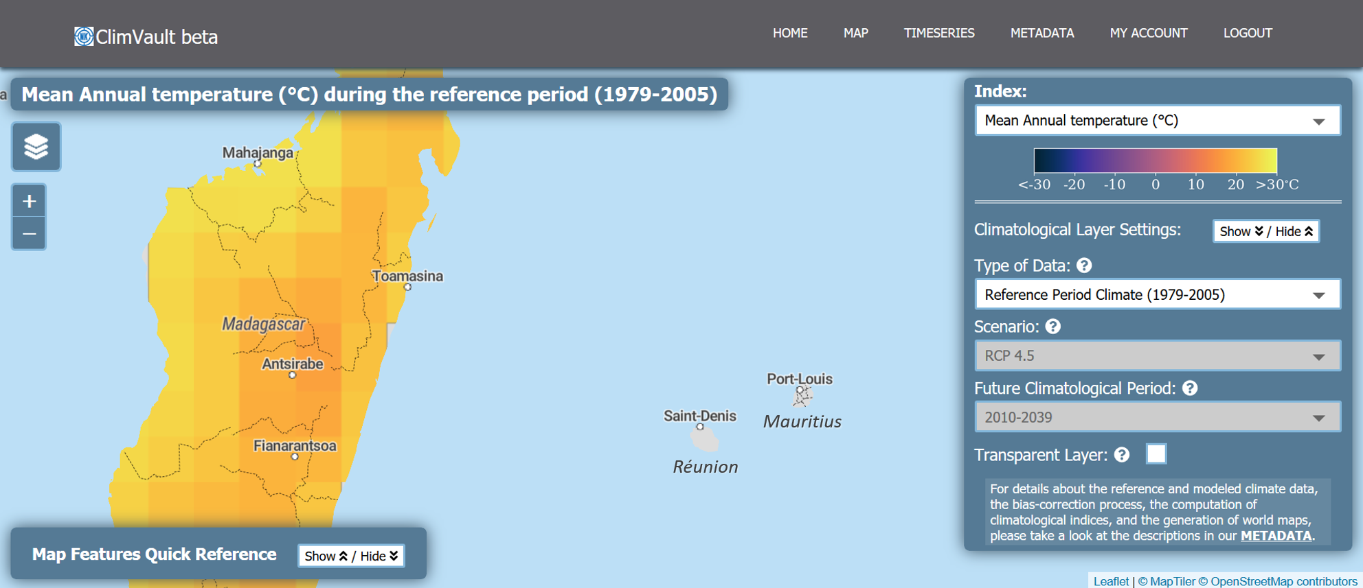
Screenshot of one of our maps showing that the extreme weather indices were not generated over Mauritius or the French Department of Réunion. Because two or four climate model grids might encounter over the islands and because the size of the islands is small compared to that of the climate model grid, the climate model simulates the grid as ocean surface.

1.2 Modeled data

The numerical climate models are tools that help scientists investigate the effects on the Earth’s climate that can be caused by the changes in the atmospheric concentration of (heat-trapping) greenhouse gases and aerosols. Within these models, which are known as global atmosphere-ocean general circulation models (AOGCMs), the complex interactions between the physical components of the climate system are approximated using mathematical equations. The capability of (AOGCMs) was further improved by including the representation of biochemical cycles. These more comprehensive models are denominated Earth System Models (ESMs, Flato et al., 2011). In ClimVault, the term climate model is generally used to refer to ESMs.

Basic structure of the recent state-of-the-art climate models (ESMs). Blue boxes show components of “standard” AOGCMs and green boxes show the components that improved the representation of biochemical cycles in ESMs.
(Ref.: Flato et al., 2013; Credits: climateurope.eu, photographs courtesy of pixabay)

The Coupled Model Intercomparison Project (CMIP) Panel is in charge of overseeing and organizing the periodical experimental protocols or phases in which climate models of several research institutions around the world participate. For generating the information that is provided in the current version of ClimVault, we used the outputs of 13 climate models participating in the CMIP Phase 5 or CMIP5 (Taylor, 2012), which are shown in the Table below.

Modeled Data Summary Table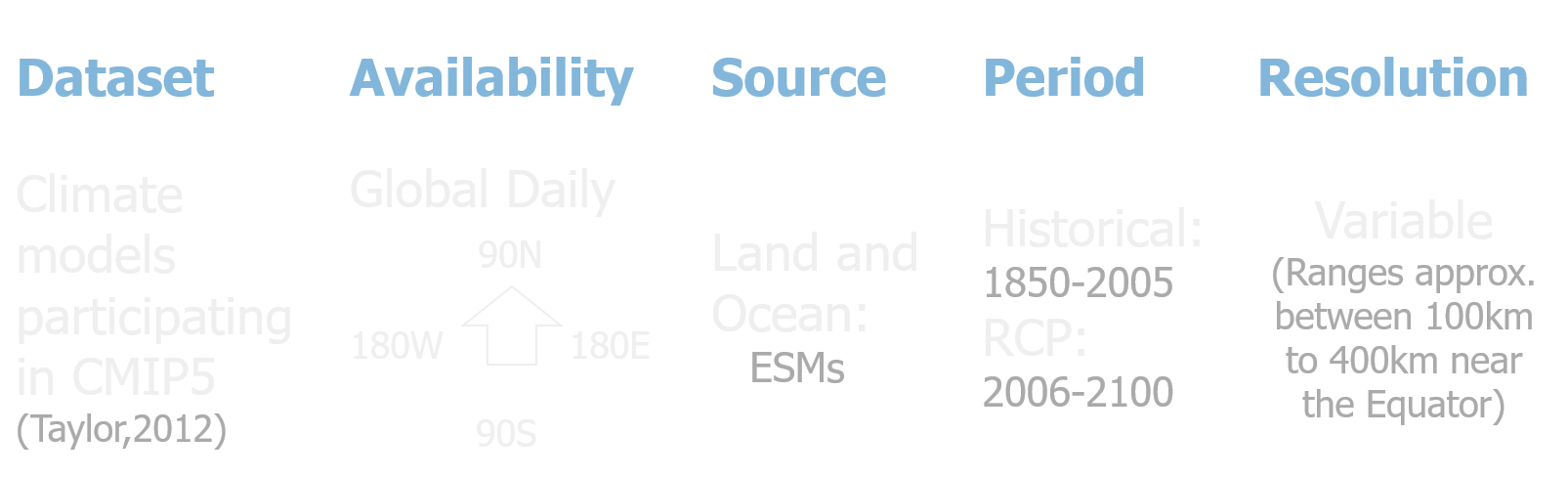

From each climate model, we utilized the long-term simulations of the “historical” and “rcp” experiments. The “historical” experiment or recent past (1850-2005) imposes changing conditions consistent with observations that include atmospheric concentrations of gases and aerosols as well as land use. The “rcp” experiments are future projections (2006-2100) forced by the Representative Concentration Pathways (RCPs; van Vuuren, 2011). There are four RCPs that lead to radiative forcing levels of 8.5, 6.0, 4.5 and 2.6 W/m², by the end of the 21st century. Radiative forcing is a quite complex term, but it basically refers to the net change in the energy balance of the Earth system due to some perturbation, like the change in the atmospheric concentration of greenhouse gases. The four RCPs are the result of an extensive literature review of experiments that used different models and assumptions about the future changes in the emissions and concentrations of greenhouse gases and air pollutants. In this way, the RCPs allow to simulate the future climate of different scenarios associated to different levels of climate policies aimed at reducing the emissions of greenhouse gases and air pollutants (these include the no-climate-policies scenarios as well).

Clicking the button that appears below opens a new tab showing the global average surface temperature change from 2006 to 2100, relative to 1986-2005, as determined by multi-model simulations (that is, the ESMs participating in the CMIP5). The graph is Figure SPM.6(a) of the “IPCC Climate Change 2014 Synthesis Report Summary for Policymakers” (IPCC, 2014). The graph shows that the multi-model mean change of the global average surface temperature by 2081-2100 is 1.8°C for the RCP4.5 (with a likely range of 1.1°C to 2.6°C) and 3.7°C for the RCP8.5 (with a likely range of 2.6°C to 4.8°C). These outcomes are the consequence of the RCP4.5 being associated to a scenario in which the emissions of greenhouse gases declines after reaching a peak around 2040 (as a probable result of climate mitigations), while the RCP8.5 is associated to a scenario in which the emissions rise persistently during the whole period.

Click HERE for GRAPH

The information available on the current version of ClimVault corresponds to the RCPs 4.5 and 8.5.

2. Data Dimensionality

The original data of the climate models participating in the CMIP are usually made available in NetCDF-format files. For near-surface atmospheric variables, these files store global data in 3 dimensions: time, latitude and longitude. Depending on the model, and due to the spatial resolution that makes the file size vary between models, the number of files and the period to which each file corresponds are different. This section details the process of extraction of the climate data from the sources’ original files and how it was spatially converted to be used in the adjustment and evaluation processes.

2.1 Spatiotemporal Extraction

To facilitate the processing of the climate data, we divided the Earth’s surface in 12 equal zones that cover 75 degrees in the latitudinal direction and 60 degrees in the longitudinal direction, as shown in the figure below.

2.2 Spatial Homogenization

3. Adjustment and Evaluation

3.1 Bias Correction

Because the climate models are merely mathematical approximations of complex physical and chemical processes, the outputs show biases when compared to observations. Therefore, the post-process of climate model outputs is applied routinely before they can be used in impact studies.

During the last decades, several bias correction methods have been proposed that range from simple corrections of the long-term mean of climate variables to more elaborate schemes aimed at correcting extreme values. Although it is difficult to assert that one method performs better than another, there have been several efforts of the scientific community to establish the requirements that bias-corrections should fulfill or the effects on the climate data that should be avoided.

In this section, we present a description of the mathematical challenge that represents the bias-correction of climate models and the details of a methodology of correction developed by our R&D center.

Objective and Challenges

ESMs are not constraint by observations of climate variables (like temperature, humidity, precipitation rate, etc.), which means that the climate models make their simulations freely. Consequently, observed and ESM-modeled climate variables are not temporally correlated. This outcome does not mean that the model is wrong; it just means that each model has its own climate variability. Consequently, if you look at the observed weather during your birthday and it happened to be raining, there is the possibility that several climate models depict a cloudy day or a sunny day. Similarly, at longer time scales, monthly or annually averaged values of the observed and modeled time series are not necessarily correlated. In other words, an unusual observed hot or wet summer may not have happened in the same year as in the climate models.

Much like the idea of a parallel universe, the Earth System Models (ESMs) can be seen as parallel Earths in which the historical land use and atmospheric concentrations of gases and aerosols are the same but the global circulation of the atmosphere evolved differently. Consequently, ESM-modeled regional extreme weather caused by atmospheric phenomena like El Niño (which occurs every 3 to 7 years approx.) or tropical cyclones (which occur several times a year) are not temporally correlated to observations.

If the outputs of climate models are supposed to be randomly different at short time scales, how do we know that they are biased and how do we correct them? To understand the answer to this question, it is necessary to understand the difference between weather and climate (explained here). While the weather is not supposed to be correlated, long-term averages, known as climatological means, should be the same. In fact, all distributional properties of the observed and the modeled time series during a long period should be equal. Because in the model the time-evolution of atmospheric concentrations of gases and aerosols is the same as the observed one, the frequency and magnitude of (extreme) weather events are equal as well. This desired outcome is possible only if we can demonstrate that observed and modeled time series are samples of the same probability distribution.

The accomplishment of the above objectives requires overcoming several mathematical challenges, which are going to be presented throughout this section, but first, let us illustrate the meaning of the two general objectives.

The following graph shows the mean daily temperature for the city of Manaus (Brazil) during the 1979-2005 period. Both the observed and the ESM-modeled time series show a similar seasonal/periodic behavior, but comparing the corresponding daily or monthly values would most likely yield random differences.

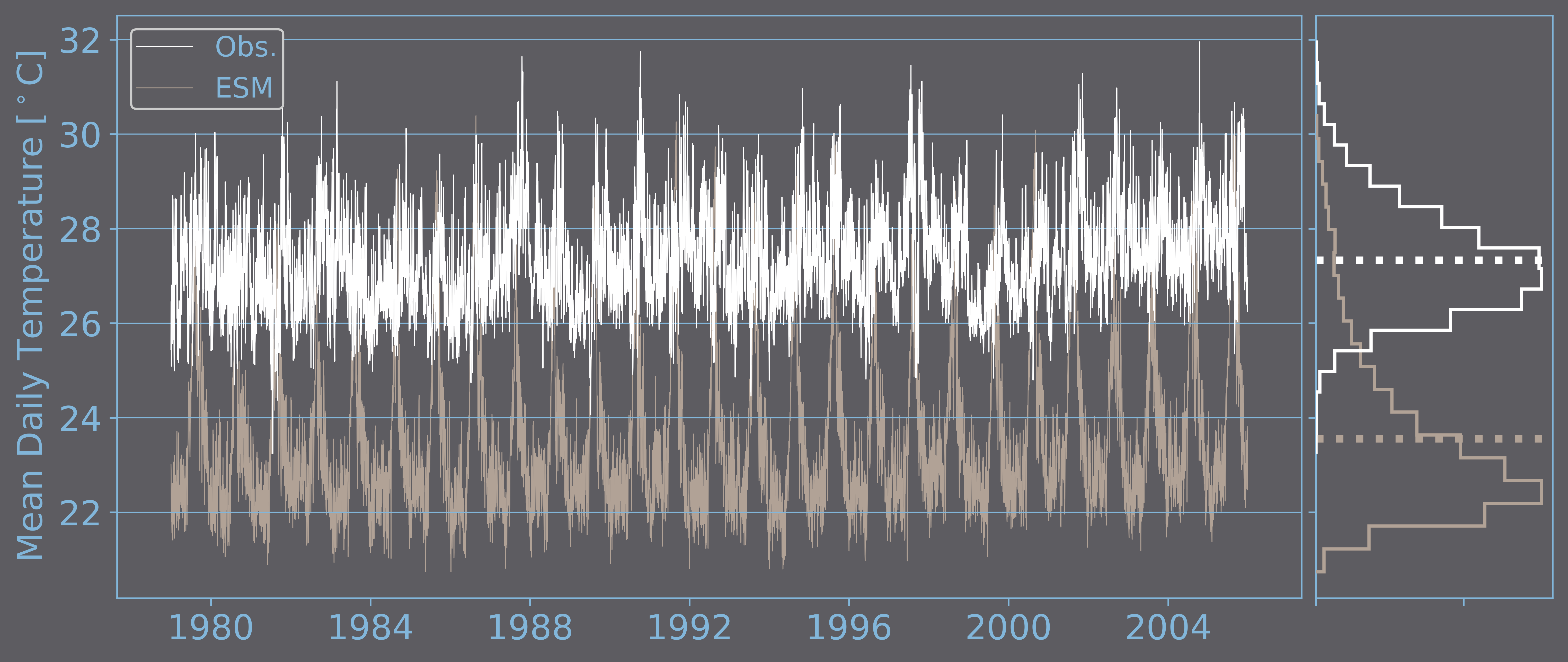
Observed (white) and ESM-modeled (beige) daily time series of mean daily temperature in °C for a grid in which the city of Manaus (Brazil) is located. Both time series correspond to the 1979-2005 period. Additionally, for each time series, the empirical density function (normalized histogram) is plotted using solid lines and the long-term average using a dotted line in the graph on the right-hand side.

If we take a look at the plots on the right-hand side of the above figure, the average of both time series have a difference of almost 4°C. This difference is one type of CLIMATE MODEL BIAS. To correct this bias, it would suffice to add it to each value of the modeled time series. The result of this simple exercise is shown in the next figure. The long-term averages of the observed and the corrected-modeled time series become equal, but the correction generates a considerable frequency of extreme temperatures that are much higher than the observed ones.

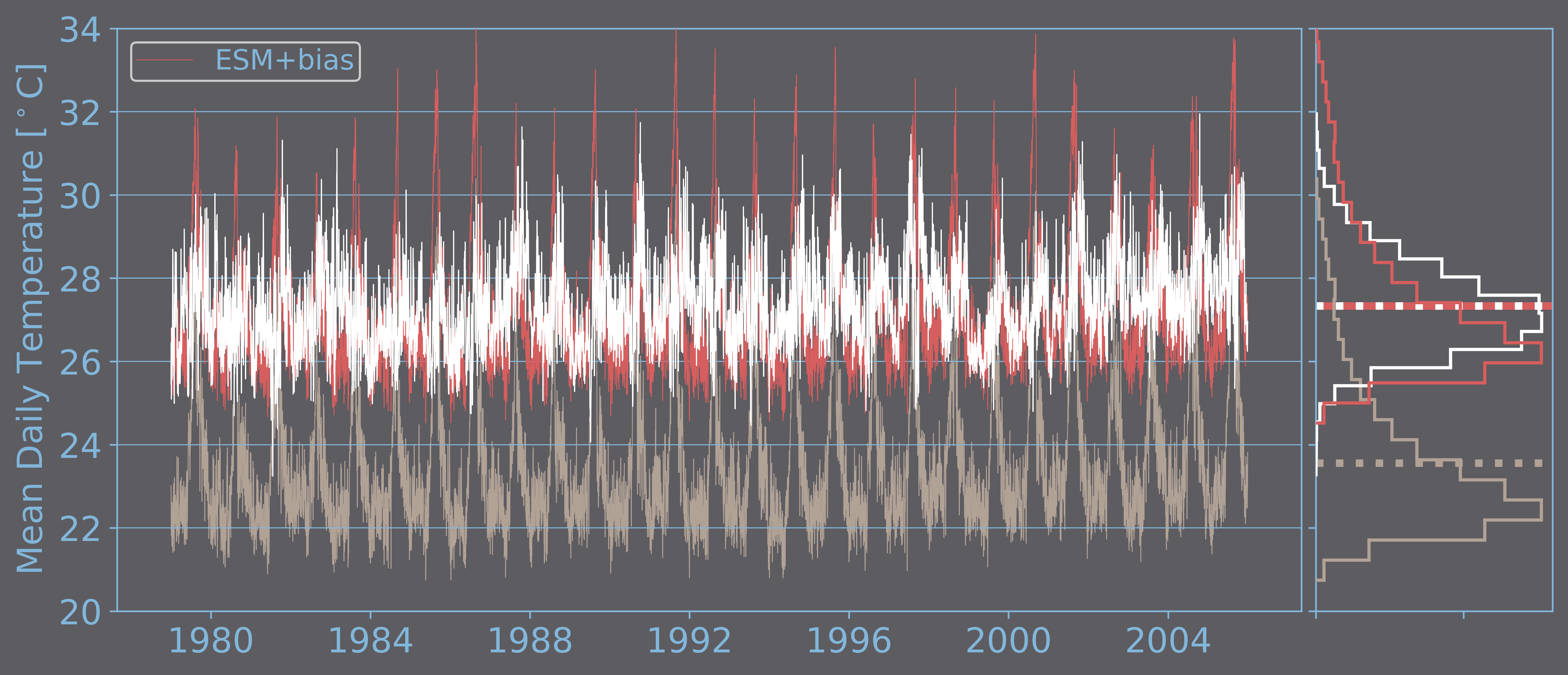
Same as the previous figure, but including the modeled time series corrected by adding the long-term-average bias (red-color lines).

Correcting by just adding the bias in the long-term average, clearly, does not make both time series samples of the same probability distributions. Considering the importance of weather extremes, as these events strongly affect and disrupt human activities, more elaborate statistical methods have been proposed aimed at correcting the extremes or tails of the empirical distributions as well. Though, to adjust probability distributions to the modeled and the observed data and then map the data of one distribution to the another can be quite challenging tasks.

The use of parametric probability distributions in the bias-correction process, like the Gaussian distribution for temperature or the Gamma distribution for precipitation intensity, is not always effective as the empirical distributions have skewness or heavy tails that cannot be modeled by these distributions. Consequently, and aided by the development of the computation capacity, methods based on non-parametric probability distributions have been developed. The objective of these methods is to practically reproduce the observed time series by dividing the observed time series in a number of intervals with equal probabilities. The next figure shows the correction using a non-parametric probability distribution that uses 10 equal intervals. In this example, a value of 25°C in the modeled time series gets mapped into a value of about 28°C (as shown with the black arrows).

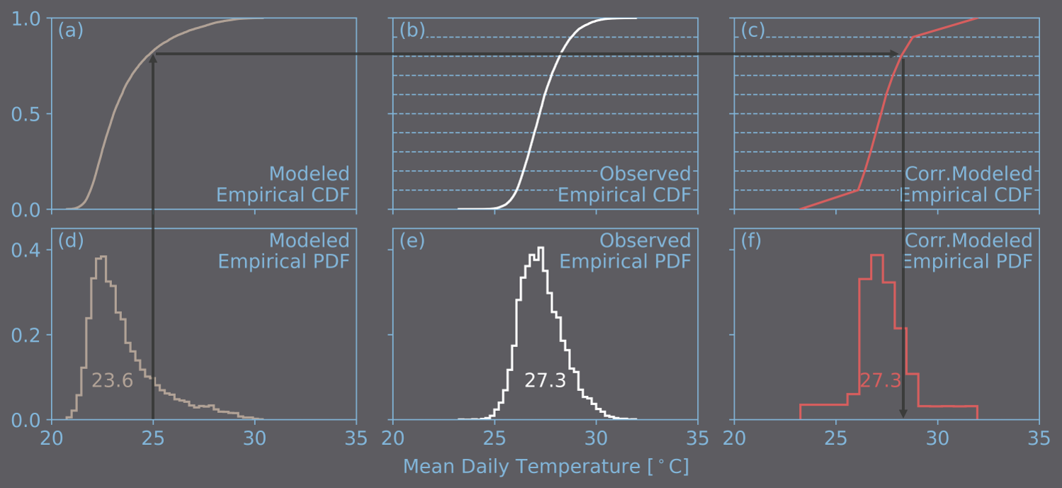
Correction of the ESM-modeled 1979-2005 time series of mean daily temperature in °C, corresponding to a grid in which the city of Manaus is located, using a non-parametric probability distribution. Graphs (a), (b) and (c) are the empirical cumulative distribution functions (CDFs) and the graphs (d), (e) and (f) are the empirical probability density functions (PDFs) of the modeled, observed and corrected-modeled time series, respectively. The non-parametric distribution function comes from dividing the observed empirical CDF in 10 equal intervals (graph (b)). Additionally, the average appears inside the histogram of each time series.

Early correction methods based on non-parametric distributions proposed using 100 intervals with equal probabilities (below figure). Aside of some differences at the tails, the empirical PDF of the observed time series looks quite similar to that of the corrected-modeled time series. To improve even more the reproduction of the observed extremes, some methodologies use non-parametric distributions with a number of intervals equal to the number of values in the observed time series, which nowadays does not represent a major computational issue.

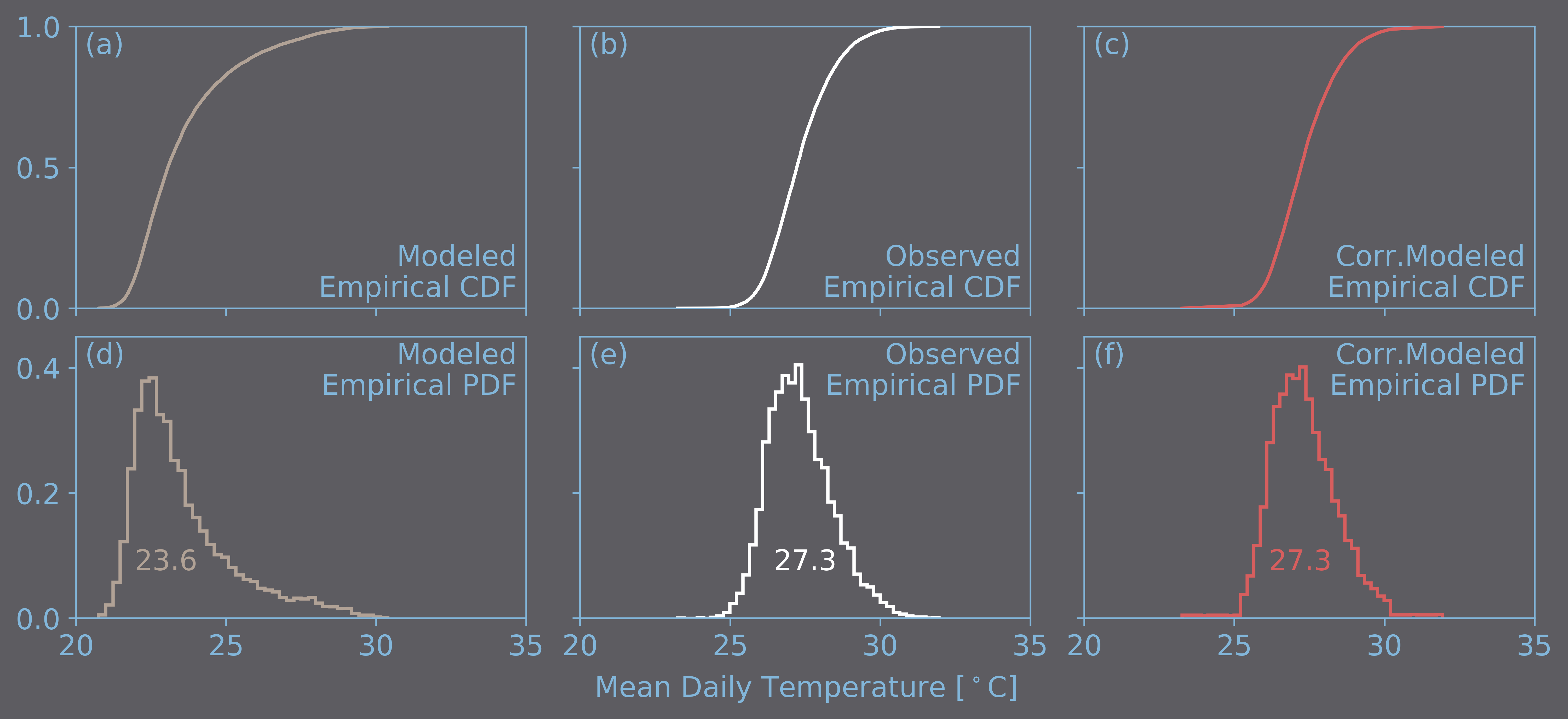
Same as the previous figure, except that the non-parametric distribution function comes from dividing the observed empirical CDF in 100 equal intervals.

The second objective (of the bias correction based on the climate model statistics) is aimed at correcting the biases in the projections of future climate. The obvious difference with the first objective is that we don’t have observations of the future. In the face of this adverse situation, the first option was to

Therefore, how to include the effects of climate change in the probability distribution of the observed time series is not only complicated but also the subject of discussion among researchers.

The correction using type of correction is flexible, which allows to include the changeHowever, trying to reproduce the observed data has some adverse consequences:

• The sampling variability of
• Because the final objective is to correct the projections of future climate, it is important that the bias-correction process does not alter the information generated by the climate models.

3.2 Regional Model Evaluation

(This section is still under construction)

4. Outputs for End-users

(This section is still under construction)

4.1 Extreme Weather Indices

4.2 City Time Series

References

• Dee D. P., Uppala S. M., Simmons A. J., Berrisford P., Poli P., Kobayashi S., et al. (2011) The ERA‐Interim reanalysis: configuration and performance of the data assimilation system. Quarterly Journal of the Royal Meteorological Society, 137(656): 553-597. doi:10.1002/qj.828
• Dutra E. (2015) Report on the current state-of-the-art Water Resources Reanalysis, Earth2observe deliverable no. D.5.1, avail-able at: http://earth2observe.eu/files/PublicDeliverables. Accessed on July 1st, 2019.
• Flato G.M. (2011) Earth System Models: An Overview. Wiley Interdisciplinary Reviews-Climate Change, 2, 783–800.
  http://dx.doi.org/10.1002/wcc.148
• Flato G., Marotzke J., Abiodun B., Braconnot P., Chou S. C., Collins W., et al. (2013) Evaluation of Climate Models. In: Climate Change 2013: The Physical Science Basis. Contribution of Working Group I to the Fifth Assessment Report of the Intergovernmental Panel on Climate Change [Stocker T. F., Qin D., Plattner G.-K., Tignor M., Allen S. K., Boschung J., et al. (eds.)]. Cambridge University Press, Cambridge, United Kingdom and New York, NY, USA.
• Harri, I., Jones P. D., Osborn T. J., and Lister D. H. (2013) Updated high-resolution grids of monthly climatic observations—The CRU TS3.10 dataset, International Journal of Climatology, 34, 623–642, doi:10.1002/joc.3711
• IPCC (2014) Climate Change 2014: Synthesis Report. Contribution of Working Groups I, II and III to the Fifth Assessment Report of the Intergovernmental Panel on Climate Change [Core Writing Team, Pachauri R. K. and Meyer L. A. (eds.)]. IPCC, Geneva, Switzerland
• Lange S. (2019) EartH2Observe, WFDEI and ERA-Interim data Merged and Bias-corrected for ISIMIP (EWEMBI). V. 1.1. GFZ Data Services. http://doi.org/10.5880/pik.2019.004
• Taylor K. E., Stouffer R. J., and Meehl G. A. (2012) An Overview of CMIP5 and the Experiment Design. Bulletin of the American Meteorological Society, 93, 485–498, https://doi.org/10.1175/BAMS-D-11-00094.1
• Schneider U., Becker A., Finger P., Meyer‐Christoffer A., Zuise M., and Rudolf B. (2013) GPCC’s new land surface precipitation climatology based on quality‐controlled in situ data and its role in quantifying the global water cycle, Theoretical and Applied Climatology, 115, 15–40, doi:10.1007/s00704‐013‐0860‐x
• van Vuuren D.P., Edmonds J., Kainuma M., Riahi K., Thomson A., Hibbard K., et al. (2011) The representative concentration pathways: an overview. Climatic Change, 109, 5–31. https://doi.org/10.1007/s10584-011-0148-z
• Weedon G. P., Balsamo G., Bellouin N., Gomes S., Best M. J., and Viterbo P. (2014) The WFDEI meteorological forcing data set: WATCH Forcing Data methodology applied to ERA-Interim reanalysis data, Water Resources Research, 50, 7505–7514, doi:10.1002/ 2014WR015638